A Journey towards Quantum World
Introduction
We like to think the universe is a sensible place. We grew up on a diet of Newtonian physics, where things stay where you put them, and if you want to get over a hill, you need enough energy to climb it. But as we peer into the subatomic machinery of reality, we find that the universe isn’t a collection of billiard balls; it’s a shivering, ghostly haze of probabilities.
Welcome to the era where the “bit”—that reliable 0 or 1—is no longer the king of the hill. We are moving beyond the bit, into a realm where particles teleport through walls and 300 atoms can hold more information than there are stars in the sky.
I. Introduction: The Death of the “Billiard Ball” Universe
The Classical Lie
For centuries, physics taught us the “Classical Lie.” It’s the comfortable analogy of a ball rolling over a hill. If the ball doesn’t have enough kinetic energy to reach the peak, it rolls back down. Simple. Logical. Completely wrong at the atomic scale.
This classical worldview, solidified by Isaac Newton in the 17th century, gave us a universe that behaved like clockwork. Given complete information about a system’s initial conditions—every position, every momentum—we could, in principle, predict its entire future with absolute certainty. Pierre-Simon Laplace, the French mathematician, famously imagined a “demon” that could know the position and motion of every atom in the universe, claiming that for such an intellect, “nothing would be uncertain and the future, just like the past, would be present before its eyes.”
This deterministic dream permeated thought for centuries. It suggested that free will might be an illusion, that the universe was a vast mechanical apparatus ticking along according to immutable laws. Cause and effect reigned supreme. If you knew enough, you could predict everything.
In our macro-world, this approximation works well enough. Boundaries are absolute. A car doesn’t suddenly phase through a cliff face. A rock thrown at a wall bounces back. But as physicists pushed deeper into the fabric of reality—first with atoms, then with their constituent particles—this elegant clockwork began to shudder and blur. The boundaries, it turned out, were merely suggestions.
The Cracks in the Clockwork
The first hints arrived in the late 19th and early 20th centuries. Max Planck, trying to solve the puzzle of how hot objects glow, discovered that energy isn’t emitted continuously but in discrete packets he called “quanta.” Then came the double-slit experiment, which delivered a blow from which classical intuition has never recovered.
When particles like electrons are fired at a barrier with two slits, they don’t behave like tiny bullets. They create an interference pattern on the detection screen—the same pattern you’d get if you fired waves at the slits. It gets stranger: even when you fire electrons one at a time, the interference pattern still emerges over time. Each electron, it seems, goes through both slits simultaneously, interfering with itself before deciding where to land. The electron doesn’t have a definite path until the moment it’s measured.
This was heresy to classical physics. An object couldn’t be in two places at once. An object couldn’t be both a particle and a wave. Yet the experiments were undeniable. The billiard ball universe was dying, and in its place, something far stranger was being born.
II. Quantum Tunneling: The Art of Walking Through Walls
Defining the Impossible
Imagine a prisoner in a cell. In a classical world, if the prisoner doesn’t have the energy to break the wall, they stay inside. The wall is an absolute barrier. In the quantum world, there is a non-zero mathematical probability that the prisoner simply… appears on the outside.
This isn’t sci-fi; it’s Quantum Tunneling, and it’s happening right now, trillions of times per second, inside your body, in the ground beneath your feet, and in the stars above your head.
The phenomenon was first predicted in the late 1920s by Friedrich Hund and then rigorously explained by George Gamow, who used it to solve a mystery plaguing nuclear physics: how do alpha particles escape from the nucleus of a radioactive atom? The nucleus is bound by the strong nuclear force, a powerful “wall” that should trap the alpha particle indefinitely. Classical physics said escape was impossible without enough energy to climb over the wall. Yet alpha particles escaped all the time. Gamow’s insight was that they didn’t climb the wall; they tunneled through it.
The Wave Function Explained
To understand tunneling, we must abandon the particle-as-billiard-ball metaphor entirely. In quantum mechanics, every particle is described by a wave function, represented by the Greek letter ψ (psi). The wave function isn’t a physical wave like sound or water; it’s a mathematical object that encodes everything knowable about the particle’s state.
Think of the wave function as a map of possibilities. Where the wave function’s magnitude is large, the particle is likely to be found. Where it’s small, the particle is unlikely to be found. Crucially, the wave function doesn’t stop at barriers—it extends into them and beyond, just as light waves extend partially into a reflective surface.
This is the heart of tunneling. When a particle encounters a barrier, its wave function doesn’t instantly drop to zero. Instead, it decays exponentially within the barrier, creating that “wave tail” on the far side. If the barrier is thin enough, the tail retains a small but non-zero amplitude. The particle isn’t “inside” the barrier in any classical sense; its wave function simply spans both sides. When we measure the particle, the wave function collapses, and we find it wherever the collapse occurs—potentially on the far side of the barrier, as if by magic.
The Mathematics of Impossibility
The probability P of a particle tunneling through a barrier is given by an exponential decay function:
P∝e−2κL
where L is the barrier width and κ depends on the particle’s mass and the barrier height. This exponential dependence is critical. Double the barrier width, and the probability doesn’t just halve—it plummets by orders of magnitude.
For an electron tunneling through a thin insulating layer in a flash memory cell, the barrier might be just a few nanometers thick. The tunneling probability is small but usable—billions of electrons tunnel every second, and we can control it. For a human attempting to tunnel through a brick wall, the barrier width is about 0.1 meters, and the mass is enormous (roughly times that of an electron). The resulting probability is so vanishingly small—on the order of 10^10^34—that you’d have to wait many trillions of times the age of the universe for it to happen once.
The universe protects its macroscopic illusions through exponential decay.
Tunneling in the Real World
Quantum tunneling isn’t a laboratory curiosity; it’s an essential feature of reality.
Stellar Fusion: The sun shines because of tunneling. Protons in the sun’s core repel each other electrostatically—they have a massive energy barrier to overcome. Classical physics says they can’t get close enough to fuse at the sun’s temperature (about 15 million Kelvin). But because of tunneling, protons occasionally slip through the barrier and fuse, releasing the energy that warms our planet. Without tunneling, the sun would be dark.
Radioactive Decay: As Gamow explained, alpha particles tunnel out of heavy nuclei. This is why uranium is radioactive and why we can use carbon dating to determine the age of archaeological artifacts.
Flash Memory: Every USB drive and SSD uses tunneling. Electrons are forced through a thin insulating layer to trap them in a “floating gate,” where their presence or absence represents a 1 or 0. The tunneling is controlled by applying voltage, which effectively “tilts” the barrier, making it thinner from the electron’s perspective.
DNA Mutations: Protons in DNA base pairs can tunnel between positions, subtly altering the genetic code. Some researchers speculate that tunneling-induced mutations may play a role in evolution and disease.
Tunneling is not a fringe effect; it’s a fundamental process woven into the fabric of physical reality.
III. The Math of the “Fuzzy” Bit
From Bits to Qubits
In a classical computer, information is stored in bits. A bit is a physical system with two distinct states—a switch that’s either on or off, a voltage that’s either high or low, a magnetic region polarized either up or down. The bit is always in one definite state. It can flip between them, but at any given moment, it’s either 0 or 1.
In a quantum computer, we use qubits. A qubit is a two-state quantum system—such as an electron’s spin (up or down) or a photon’s polarization (horizontal or vertical). But because qubits obey quantum mechanics, they can exist in a superposition of both states simultaneously.
The Qubit Formula
The state of a qubit is represented by the formula:
∣ψ⟩=α∣0⟩+β∣1⟩
Here, α and β are complex numbers called probability amplitudes. The squared magnitudes |α|² and |β|² give the probabilities of measuring the qubit in state |0⟩ or |1⟩, respectively. The qubit exists in a superposition of both |0⟩ and |1⟩ simultaneously—not as a statistical mixture, but as a coherent blend.
This is difficult to grasp because nothing in our macroscopic experience prepares us for it. A classical bit is like a coin resting on a table: it’s either heads or tails. A qubit is like a coin spinning in the air: it’s not heads or tails, but a blur of both possibilities. Unlike the spinning coin, however, the qubit isn’t secretly in one state while we’re not looking. The information of “which state” simply doesn’t exist until measurement. The qubit inhabits the boundary between possibilities.
The Bloch Sphere
Physicists visualize qubit states using the Bloch sphere, a mathematical representation where any point on the sphere’s surface corresponds to a possible pure state of a single qubit.
The north pole represents |0⟩, the south pole represents |1⟩, and every other point represents a superposition. The equator contains states like (equal superposition) and (|0⟩ – |1⟩)/√2 (equal superposition with opposite phase). The angles describe the relative weight of |0⟩ vs |1⟩ and the phase difference between them.
This geometric representation reveals something profound: a qubit doesn’t just have a “how much” property (amplitude) but also a “relationship” property (phase). Phase is invisible in classical probabilities but crucial in quantum computing—it’s what allows interference between different computational paths.
The Born Rule: Why It All Adds Up
The connection between the abstract wave function and measurable reality is given by the Born Rule, named after physicist Max Born:
∣α∣2+∣β∣2=1
The total probability must sum to 1—the particle must be somewhere when measured. This is the mathematical anchor in the storm of quantum possibility.
Born received the Nobel Prize for this insight, which fundamentally changed how we understand reality. Before Born, physicists hoped the wave function might represent a real, physical wave—that the particle was somehow “smeared out” in space. Born showed that the wave function represents knowledge about the particle, not the particle itself. The particle remains point-like; it’s the probability of finding it that spreads like a wave.
This was deeply unsettling. Einstein wrote to Born: “The theory yields a lot, but it hardly brings us closer to the Old One’s secrets. I, in any case, am convinced He does not throw dice.” Yet decades of experiments have confirmed Born’s interpretation: the universe, at its most fundamental level, is probabilistic.
Multiple Qubits and the Tensor Product
When we have multiple qubits, the state space grows exponentially. A two-qubit system isn’t just two independent qubits; it’s a combined system described by a state like:
∣ψ⟩=α00∣00⟩+α01∣01⟩+α10∣10⟩+α11∣11⟩
With two qubits, we need four probability amplitudes. With three qubits, we need eight. With n qubits, we need 2^n amplitudes. This exponential scaling is the source of quantum computing’s power—and its challenge. To simulate a 300-qubit system classically, you’d need to store and manipulate 2^300 complex numbers, a task vastly beyond any conceivable classical computer.
IV. Inhabiting the State (The Secret Sauce)
Simulation vs. Reality
The biggest misconception about quantum computers is that they are just “faster” classical computers. They aren’t. They operate on a fundamentally different logic.
Classical computers calculate math. They take inputs, run them through logic gates, and spit out an answer. Even when simulating physical systems, they remain external—they model reality without participating in it.
Quantum computers become the math.
When a quantum computer solves a molecule’s energy state, it isn’t simulating the molecule; it is using its own quantum states to mirror the molecule’s behavior. The electrons in the computer’s qubits interact according to the same quantum rules as the electrons in the real molecule. The computation isn’t an analogy for physics; it is physics.
As Richard Feynman famously said in 1981, “Nature isn’t classical, dammit, and if you want to make a simulation of nature, you’d better make it quantum mechanical.” Feynman recognized that classical computers would always struggle with quantum systems because they’re playing a game with the wrong rules. To understand the quantum world, you need to speak its language.
The Power of 300
To understand the scale of quantum advantage, consider this:
- 2 Qubits can represent 4 states simultaneously.
- 10 Qubits can represent 1,024 states.
- 50 Qubits can represent over 1 quadrillion states (2^50 ≈ 1.1 × 10^15).
- 300 Qubits can represent 2^300 states.
That number——is approximately . The observable universe contains roughly atoms. A relatively small quantum machine can process a landscape of possibilities—a “state space”—that is larger than physical reality itself.
This doesn’t mean the quantum computer contains more information than the universe; information is still physical, and the qubits themselves are real physical systems. But the number of distinct computational paths it can explore simultaneously exceeds the number of particles in existence. It navigates a mathematical space whose size dwarfs physical reality.
This is what “Quantum Supremacy” means: not that quantum computers can solve any problem faster than classical ones, but that there exist problems they can solve that are practically impossible for any classical computer, no matter how powerful.
The Energy Snap
The moment we measure a qubit, the superposition collapses. The “fuzziness” snaps into a binary 0 or 1. This is the Energy Snap—the violent reduction of infinite possibility to a single, stark fact.
The measurement problem—how and why collapse occurs—remains one of the deepest mysteries in physics. Some interpretations (like the Copenhagen interpretation) treat collapse as a fundamental process: the wave function simply chooses a result when measured. Others (like many-worlds) deny collapse entirely, claiming that all possibilities continue to exist in branching universes. Still others (like Bohmian mechanics) insist the particle has a definite trajectory all along, guided by a “pilot wave.”
What’s experimentally certain is that quantum superpositions are extraordinarily fragile. The environment “observes” the qubit, forcing it to decohere and join the boring, classical world. Any interaction with the outside world—a stray photon, a thermal vibration, a cosmic ray—can trigger collapse. This transition—from quantum wave to classical fact—is the hardest part of building these machines.
V. The Quantum Toolbox: Gates and States
Quantum Logic
In classical computing, we have logic gates: AND, OR, NOT, XOR, and so on. These gates take bits as input and produce deterministic outputs. They’re built from transistors and follow Boolean algebra.
In quantum computing, we have quantum gates. These are unitary transformations—reversible operations that rotate qubit states on the Bloch sphere. Unlike classical gates (except NOT), quantum gates are always reversible. This reversibility is fundamental: quantum evolution is unitary, meaning information is never destroyed, only transformed.
Single-Qubit Gates
| Gate | Name | Matrix | Function | ||||||
|---|---|---|---|---|---|---|---|---|---|
| I | Identity | [[1,0],[0,1]] | Does nothing; leaves the qubit unchanged. | ||||||
| X | Pauli-X | [[0,1],[1,0]] | The quantum NOT gate. Flips | 0⟩ to | 1⟩ and | 1⟩ to | 0⟩. Equivalent to a rotation around the X-axis by π radians. | ||
| Y | Pauli-Y | [[0,-i],[i,0]] | Rotates around the Y-axis; introduces complex phases. | ||||||
| Z | Pauli-Z | [[1,0],[0,-1]] | Flips the phase of | 1⟩ while leaving | 0⟩ unchanged. | ||||
| H | Hadamard | (1/√2)[[1,1],[1,-1]] | Creates superposition. Turns | 0⟩ into ( | 0⟩+ | 1⟩)/√2 and | 1⟩ into ( | 0⟩- | 1⟩)/√2. The most important gate for creating quantum parallelism. |
The Hadamard gate deserves special attention. It takes a definite state and produces an equal superposition—a qubit that’s perfectly balanced between 0 and 1. When applied to multiple qubits in parallel, it creates a superposition of all possible computational basis states simultaneously. This is how quantum computers achieve parallelism: with a single layer of Hadamard gates, an n-qubit register enters a superposition of all 2^n possible states.
Two-Qubit Gates
The real power of quantum computing emerges when qubits interact. The fundamental two-qubit gate is the Controlled-NOT (CNOT):
| Gate | Name | Matrix | Function | |
|---|---|---|---|---|
| CNOT | Controlled-NOT | [[1,0,0,0],[0,1,0,0],[0,0,0,1],[0,0,1,0]] | Flips the target qubit if and only if the control qubit is | 1⟩. |
The CNOT gate is the quantum equivalent of the classical XOR, but with an important difference: it’s reversible. Given the output, you can reconstruct the input. This reversibility is essential for quantum computing.
CNOT, combined with single-qubit gates, is universal for quantum computation—any quantum operation can be decomposed into CNOTs and single-qubit rotations.
The Bell State: Maximal Entanglement
When you apply a Hadamard gate followed by a CNOT gate to two qubits initially in |00⟩, you create a Bell State:
∣Φ+⟩=2∣00⟩+∣11⟩
This is “Entanglement”—what Einstein called “spooky action at a distance.” Two entangled qubits are linked in a way that defies classical intuition. They are no longer two separate objects with independent properties; they are a single, two-part system whose properties are undefined until one of them is forced to choose.
If you measure the first qubit and find it to be |0⟩, you instantly know, with 100% certainty, that its entangled partner is |0⟩—even if it’s on the other side of the galaxy. If you find the first to be |1⟩, the second is |1⟩. The correlation is perfect and instantaneous.
This “instantaneous” aspect troubled Einstein deeply. Special relativity says nothing can travel faster than light, yet entanglement seems to transmit information across any distance instantly. The resolution is subtle: entanglement doesn’t allow faster-than-light communication because you can’t control which outcome you get. The correlation is only visible after comparing measurement results using classical communication. Entanglement creates correlations stronger than any classical system can produce, but it doesn’t violate relativity.
The No-Cloning Theorem
An important consequence of quantum mechanics is the no-cloning theorem: you cannot make a perfect copy of an unknown quantum state. If you have a qubit in an unknown superposition, there’s no operation that will produce two identical qubits in that same state while preserving the original.
This theorem, proved in 1982 by Wootters, Zurek, and Dieks, has profound implications. It underlies the security of quantum cryptography—an eavesdropper can’t copy quantum states without disturbing them. It also means quantum error correction must work differently than classical error correction, using entanglement to spread quantum information across multiple physical qubits.
VI. Algorithms: Rigging the Results
The Problem of Measurement
If measuring a quantum computer just gives you a random 0 or 1, how is it useful? This is the central challenge of quantum algorithm design. A naive quantum computer would be nothing more than a very expensive random number generator.
The trick is Interference.
Think of noise-canceling headphones. They sample ambient sound and produce an inverted wave that interferes destructively with the noise, canceling it out. Meanwhile, the music you want to hear is amplified through constructive interference.
Quantum algorithms do the same with probability amplitudes. They manipulate the phases of computational paths so that wrong answers interfere destructively (canceling each other) while right answers interfere constructively (amplifying each other). When you finally measure, the probability of seeing a correct answer is dramatically enhanced.
Quantum Parallelism
The first insight is that quantum computers can evaluate a function f(x) for many x simultaneously. By putting input qubits in superposition, applying the unitary that computes f, you get:
∑x∣x⟩∣0⟩→∑x∣x⟩∣f(x)⟩
You’ve computed f(x) for all x in a single step. This is quantum parallelism.
But parallelism alone isn’t enough—you still face the measurement problem. If you measure immediately, you’ll just get one random (x, f(x)) pair, no better than a classical computer. The art is to transform the quantum state before measurement, using interference to extract global properties of f.
Grover’s Algorithm: The Needle in the Haystack
Suppose you have an unsorted database of N items, and you want to find one specific item. Classically, you’d have to check items one by one—on average, N/2 checks before success. For N = 1 million, that’s 500,000 checks.
Grover’s Algorithm, discovered by Lov Grover in 1996, uses quantum interference to find the target in only about √N steps. For 1 million items, that’s just 1,000 steps—a quadratic speedup.
The algorithm works by repeatedly applying two operations:
- An “oracle” that flips the phase of the target state
- A “diffusion” operator that inverts amplitudes about the average
Initially, all states have equal amplitude. The oracle marks the target by flipping its phase (making it negative). The diffusion operator then amplifies states with negative phase while suppressing others. After about √N iterations, the target’s amplitude is near 1, and measurement reveals it with high probability.
Grover’s algorithm is optimal—no quantum algorithm can do unstructured search faster than √N. It demonstrates that quantum computers can provide polynomial speedups for certain problems, though not the exponential speedup of Shor’s algorithm.
Shor’s Algorithm: The Quantum Apocalypse
This is why governments are sweating. Most of our modern encryption (RSA) relies on the fact that it’s nearly impossible for classical computers to find the prime factors of a massive number. Multiplying two large primes is easy; finding the primes given the product is hard. The security of online banking, encrypted email, and state secrets rests on this asymmetry.
Shor’s Algorithm, discovered by Peter Shor in 1994, shatters this assumption. It doesn’t try to “guess” the factors through brute force. Instead, it uses the wave nature of qubits to find the period of a mathematical function related to the number being factored.
The algorithm exploits a connection between factoring and period-finding. For a given number N to factor, choose a random a less than N. Consider the function f(x) = a^x mod N. This function is periodic—it repeats after some period r. Once you find r, simple algebra reveals the factors of N.
Finding r classically is hard. But with a quantum computer:
- Create a superposition of all x
- Compute f(x) into a second register
- Measure the second register (collapsing the first into a superposition of x with the same f(x))
- Apply the Quantum Fourier Transform to reveal the period r
The Quantum Fourier Transform is the heart of the algorithm. It extracts the period from the quantum state through interference, just as a classical Fourier transform extracts frequencies from a signal. The result is that a quantum computer can find r in polynomial time—exponentially faster than any known classical algorithm.
When a sufficiently powerful quantum computer arrives, every encrypted email, bank transfer, and state secret currently protected by RSA will be laid bare. This isn’t a faster brute-force attack; it’s a fundamental end-run around the logic that keeps our secrets safe.
Quantum Fourier Transform
The Quantum Fourier Transform (QFT) deserves special mention. It’s the quantum equivalent of the discrete Fourier transform, mapping a quantum state to its frequency components. Remarkably, the QFT can be implemented exponentially faster than the classical Fast Fourier Transform—using only O((log N)²) gates instead of O(N log N).
The QFT is the engine behind Shor’s algorithm and many other quantum algorithms. It demonstrates how quantum computers excel at problems involving hidden periodic structure—a clue that quantum mechanics is particularly suited to certain mathematical tasks.
VII. Physical Implementations: Building the Impossible
The Qubit Zoo
There’s no single way to build a qubit. Different approaches have different trade-offs, and it’s not yet clear which will win in the long run.
Superconducting Qubits: Currently the leading platform, used by Google and IBM. These are tiny superconducting circuits that behave like artificial atoms. They’re fabricated using standard semiconductor techniques, making them relatively scalable. However, they require dilution refrigerators to reach millikelvin temperatures, and their coherence times (how long they maintain quantum states) are measured in microseconds.
Trapped Ions: Used by IonQ and Honeywell. Individual ions are trapped using electric fields and manipulated with lasers. They have exceptional coherence times (seconds to minutes) and high-fidelity operations, but scaling to many qubits is challenging—each ion needs its own laser beams.
Photonic Qubits: Qubits encoded in photons. They operate at room temperature and couple naturally to fiber optics, making them promising for quantum communication. However, photons don’t interact easily, making two-qubit gates difficult.
Spin Qubits: Qubits encoded in the spin of electrons or nuclei in semiconductors like silicon. They leverage existing semiconductor manufacturing, potentially scaling like classical chips. But they’re tiny and difficult to control individually.
Topological Qubits: A theoretical approach pursued by Microsoft. These would store information in non-local properties of quasiparticles called anyons, making them inherently resistant to decoherence. So far, they remain unproven experimentally.
The Enemy: Decoherence
Qubits are incredibly fragile. A single photon, a tiny change in temperature, or a slight vibration can cause Decoherence—the loss of quantum information to the environment. It’s like trying to keep a perfectly still pond absolutely silent; the slightest ripple destroys the reflection.
Decoherence occurs because qubits inevitably interact with their environment. That interaction entangles the qubit’s state with the environment’s state. From the qubit’s perspective, information leaks out—the superposition collapses into a mixture, and quantum coherence is lost.
To prevent this, we keep quantum processors at temperatures colder than outer space (about 0.01 Kelvin, colder than the cosmic microwave background). We shield them from magnetic fields with multiple layers of mu-metal. We isolate them from vibrations using sophisticated suspension systems. We even worry about cosmic rays—a single high-energy particle can disrupt an entire calculation.
The slightest whisper from the environment collapses the beautiful wave of possibility into mundane, classical fact.
The Solution: Logical Qubits
To build a computer that can actually run Shor’s Algorithm, we need error correction. Quantum error correction is fundamentally different from classical error correction because you can’t just copy qubits (no-cloning theorem) and measurements disturb quantum states.
Instead, quantum error correction encodes one “logical” qubit across many “physical” qubits using entanglement. Information is distributed non-locally—no single physical qubit holds the complete information.
The most promising approach is the surface code, which arranges qubits on a 2D grid. By repeatedly measuring certain stabilizer operators, errors can be detected and corrected. Current estimates suggest we need roughly 1,000 physical qubits to create one “perfect” logical qubit.
This is the hidden challenge behind the headlines. A machine with 50 perfect qubits is impressive, but we might need a machine with 10 million physical qubits to break modern encryption.
The NISQ Era
We are currently in the NISQ era (Noisy Intermediate-Scale Quantum). The machines exist—Google’s Sycamore, IBM’s Eagle, and others—but they are “leaky.” They have dozens to hundreds of qubits, but with significant error rates and limited connectivity.
NISQ computers may never run Shor’s algorithm, but they’re not useless. Researchers are exploring hybrid quantum-classical algorithms like the Variational Quantum Eigensolver (VQE) and the Quantum Approximate Optimization Algorithm (QAOA). These use short quantum circuits combined with classical optimization to tackle problems in chemistry, materials science, and optimization.
The NISQ era is teaching us how to build and control quantum systems at scale, even if the machines themselves are too noisy for full-scale fault-tolerant computation.
VIII. Implications and the Future
Q-Day
“Q-Day” is the hypothetical date when a quantum computer becomes powerful enough to break RSA-2048. It hasn’t happened yet, but the race is on to develop Post-Quantum Cryptography (PQC)—math problems that are hard even for quantum computers to solve.
The National Institute of Standards and Technology (NIST) is leading an international effort to standardize PQC algorithms. Candidates include lattice-based cryptography, code-based cryptography, and multivariate cryptography. These systems don’t rely on factoring or discrete logarithms, making them resistant to Shor’s algorithm.
Beyond Cryptography
While cryptography grabs headlines, quantum computing’s impact may be broader in other areas:
Materials Science: Quantum computers could simulate complex molecules and materials exactly, enabling the design of room-temperature superconductors, more efficient solar cells, better batteries, and novel pharmaceuticals. This isn’t just faster computation—it’s a new way of understanding matter.
Chemistry: Understanding enzyme reactions, designing catalysts, and predicting molecular properties could revolutionize chemical engineering. The Haber process for fertilizer production, which feeds billions of people, could be made dramatically more efficient.
Machine Learning: Quantum machine learning algorithms might find patterns in data that classical algorithms miss.
Fundamental Physics: Quantum simulators could help us understand high-temperature superconductivity, quantum magnetism, and even aspects of quantum gravity.
The Philosophical Shift
The journey from Quantum Tunneling—a weird fluke of subatomic particles—to the Quantum Apocalypse is really a journey of understanding.
This shift is as profound as the Copernican revolution. Copernicus showed us that Earth isn’t the center of the cosmos. Darwin showed us we’re not separate from the animal kingdom. Quantum mechanics shows us that reality isn’t made of solid, deterministic matter—it’s made of relationships, probabilities, and possibilities.
The universe doesn’t speak the language of billiard balls and clockwork. It speaks the language of waves, interference, and infinite possibilities.
The Ethical Dimension
With great power comes great responsibility. A technology that can break encryption, simulate molecules, and navigate state spaces larger than the universe carries profound ethical implications.
Who gets access to quantum computers? How do we ensure they’re used for benefit rather than harm? What happens to privacy in a post-quantum world? How do we prevent a quantum arms race?
These questions have no easy answers.
IX. Conclusion: A New Language for Nature
We are moving away from the era of forcing nature to act like a machine and into the era of building machines that act like nature.
The classical worldview gave us incredible power—steam engines, electricity, computers, rockets. But it also gave us a false sense of separation from the cosmos. We stood outside nature, manipulating it, forcing it to obey our rules.
Quantum mechanics dissolves this separation. We’re not external observers; we’re participants. The act of measurement changes what’s measured. The information we seek isn’t waiting to be discovered—it’s created through our interaction with reality.
The universe isn’t made of things. It’s made of possibilities. And for the first time, we’re learning how to explore them.